ST 558 Project 3: Lifestyle Analysis Report
Suyog Dharmadhikari; Bennett McAuley 2022-11-02
Introduction
The goal of this report is to create and compare predictive models using Online News Popularity data from the UCI Machine Learning Repository.
This data contains information about articles published by Mashable over a period of two years–specifically the statistics associated with them.
The purpose of this analysis is to use linear regression and ensemble
tree-based methods to predict the number of shares–our target
variable–subset by data channel. For more details about these methods,
see the Modeling section.
According to the data description, there are 39,797 observations and 61 variables present. 58 of them are predictors, but using all of them would be inefficient and show glaring redundancies. Instead, the ones that will be used were chosen intuitively–what might encourage a user to share an article, what underlying forces may influence them, and what would make for good exploratory analysis:
average_token_length- Average length of the words in the contentavg_negative_polarity- Avg. polarity of negative wordsglobal_rate_positive_words- Rate of positive words in the contentglobal_sentiment_polarity- Text sentiment polarityglobal_subjectivity- Text subjectivityis_weekend- Was the article published on the weekend?kw_avg_max- Best keyword (avg. shares)kw_avg_min- Worst Keyword (avg. shares)kw_max_max- Best keyword (max shares)kw_min_min- Worst keyword (min shares)n_non_stop_words- Rate of non-stop words in the contentn_tokens_content- Number of words in the contentn_tokens_title- Number of words in the titlen_unique_tokens- Rate of unique words in the contentnum_hrefs- Number of linksnum_imgs- Number of imagesnum_self_hrefs- Number of links to other articles published by Mashablenum_videos- Number of videosself_reference_avg_shares- Avg. shares of referenced articles in Mashabletitle_sentiment_polarity- Title polarityweekday_is_monday- Was the article published on a Monday?weekday_is_tuesday- Was the article published on a Tuesday?weekday_is_wednesday- Was the article published on a Wednesday?weekday_is_thursday- Was the article published on a Thursday?weekday_is_friday- Was the article published on a Friday?weekday_is_saturday- Was the article published on a Saturday?weekday_is_sunday- Was the article published on a Sunday?
Which we store in a vector for fast retrieval:
news.vars <- c('n_tokens_title', 'n_tokens_content', 'n_non_stop_words', 'num_hrefs',
               'num_self_hrefs', 'num_imgs', 'num_videos', 'average_token_length',
               'kw_max_max', 'kw_min_min', 'kw_avg_max', 'kw_avg_min',
               'self_reference_avg_sharess','is_weekend', 'global_subjectivity', 'global_sentiment_polarity',
               'global_rate_positive_words', 'avg_negative_polarity', 'n_unique_tokens', 'title_sentiment_polarity',
               'weekday_is_sunday', 'weekday_is_monday', 'weekday_is_tuesday', 'weekday_is_wednesday',
               'weekday_is_thursday', 'weekday_is_friday', 'weekday_is_saturday'
               )
The Data
For this analysis, we will consider a single source for the data channel. In other words, we subset the data to the Lifestyle channel.
So, we read in the data, perform the filter, and convert is_weekend
into a binary factor:
news <- read_csv("OnlineNewsPopularity.csv")
## Rows: 39644 Columns: 61
## ── Column specification ───────────────────────────────────────────────────────────────────────────
## Delimiter: ","
## chr  (1): url
## dbl (60): timedelta, n_tokens_title, n_tokens_content, n_unique_tokens, n_non_stop_words, n_non...
##
## ℹ Use `spec()` to retrieve the full column specification for this data.
## ℹ Specify the column types or set `show_col_types = FALSE` to quiet this message.
fltr <- paste0("data_channel_is_", params$channel)

news.tbl <- news %>% filter(get(fltr) == 1) %>%
  select(all_of(news.vars), shares) %>%
  mutate(is_weekend = as.factor(is_weekend))

head(news.tbl)
## # A tibble: 6 × 28
## n_token…¹ n_tok…² n_non…³ num_h…⁴ num_s…⁵ num_i…⁶ num_v…⁷ avera…⁸ kw_ma…⁹ kw_mi…˟ kw_av…˟ kw_av…˟
## <dbl> <dbl> <dbl> <dbl> <dbl> <dbl> <dbl> <dbl> <dbl> <dbl> <dbl> <dbl>
## 1 8 960 1.00 21 20 20 0 4.65 0 0 0 0
## 2 10 187 1.00 7 0 1 0 4.66 0 0 0 0
## 3 11 103 1.00 3 1 1 0 4.84 0 0 0 0
## 4 10 243 1.00 1 1 0 0 4.38 0 0 0 0
## 5 8 204 1.00 7 2 1 0 4.67 0 0 0 0
## 6 11 315 1.00 4 4 1 0 4.38 0 0 0 0
## # … with 16 more variables: self_reference_avg_sharess <dbl>, is_weekend <fct>,
## # global_subjectivity <dbl>, global_sentiment_polarity <dbl>, global_rate_positive_words <dbl>,
## # avg_negative_polarity <dbl>, n_unique_tokens <dbl>, title_sentiment_polarity <dbl>,
## # weekday_is_sunday <dbl>, weekday_is_monday <dbl>, weekday_is_tuesday <dbl>,
## # weekday_is_wednesday <dbl>, weekday_is_thursday <dbl>, weekday_is_friday <dbl>,
## # weekday_is_saturday <dbl>, shares <dbl>, and abbreviated variable names ¹n_tokens_title,
## # ²n_tokens_content, ³n_non_stop_words, ⁴num_hrefs, ⁵num_self_hrefs, ⁶num_imgs, ⁷num_videos, …
Summarizations
Now that our data has been manipulated and filtered, we can perform a simple EDA.
Summary Statistics
First and foremost, we want to know what range of values we might expect
when predicting for shares. The following table shows basic summary
statistics about the variable:
s <- summary(news.tbl$shares)

tibble(var = 'shares', min = s[1], max = s[6], mean = s[3], stddev = sd(news.tbl$shares))
## # A tibble: 1 × 5
##   var    min     max     mean    stddev
##   <chr>  <table> <table> <table>  <dbl>
## 1 shares 28      208300  1700     8885.
If the maximum is tremendously larger in scale than the mean, then it is very likely an outlier. If the standard deviation is larger than the mean, then the number of shares varies greatly. Furthermore, the higher it is, the more disperse they are from the mean. The inverse also applies for a smaller standard deviation (i.e. the smaller, the less disperse).
It would also be good to know relationships between some of the
variables present–and not just to shares. Observe the following
correlation matrix of variables related to content sentiment. A value of
0 indicates no correlation and 1 indicates perfect correlation. The
closer a value is to 1(+/-), the stronger the relationship is. The
closer to 0, the weaker.
c <- news.tbl %>%
  select(avg_negative_polarity,
         global_rate_positive_words,
         global_sentiment_polarity,
         global_subjectivity,
         shares)

round(cor(c),2)
##                            avg_negative_polarity global_rate_positive_words
## avg_negative_polarity                       1.00                      -0.07
## global_rate_positive_words                 -0.07                       1.00
## global_sentiment_polarity                   0.22                       0.58
## global_subjectivity                        -0.33                       0.38
## shares                                     -0.03                      -0.01
##                            global_sentiment_polarity global_subjectivity shares
## avg_negative_polarity                           0.22               -0.33  -0.03
## global_rate_positive_words                      0.58                0.38  -0.01
## global_sentiment_polarity                       1.00                0.39  -0.02
## global_subjectivity                             0.39                1.00   0.02
## shares                                         -0.02                0.02   1.00
The new variable popularity is set up so that news is considered
popular if it receives more shares than the median shares. Otherwise,
it is considered unpopular.table() gives details about count of
popular and unpopular news.
news.tbl$popularity <- ifelse(news.tbl$shares < mean(news.tbl$shares),
                              "Unpopular", "Popular")

table(news.tbl$popularity)
##
##   Popular Unpopular
##       469      1630
The contingency table below depicts the relationship between the popularity of a news channel and whether or not it was published on the weekend. It informs us whether or not popular news was published over the weekend. Whether or not unpopular news was published over the weekend.
table(news.tbl$popularity,news.tbl$is_weekend)
##
##                0    1
##   Popular    359  110
##   Unpopular 1348  282
Plots
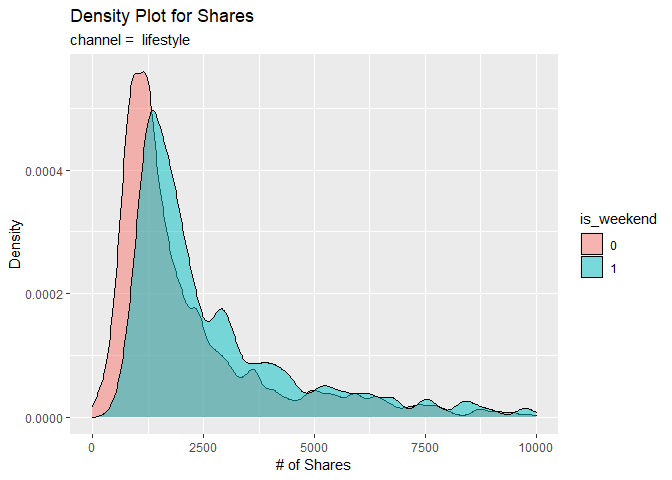
For visual analysis, we first construct a density plot to compare the
densities of shares between the weekend (is_weekend = 1) and
weekdays (is_weekend = 0). Observe the patterns generated for
similarities and/or differences.
g <- ggplot(data = news.tbl, aes(x = shares))

g + geom_density(adjust = 0.5, alpha = 0.5, aes(fill = is_weekend)) +
  xlim(0, 10000) +
  scale_y_continuous(labels = scales::comma) +
  labs(title = "Density Plot for Shares",
       subtitle = paste("channel = ", params$channel),
       x = "# of Shares",
       y = "Density")
## Warning: Removed 141 rows containing non-finite values (stat_density).
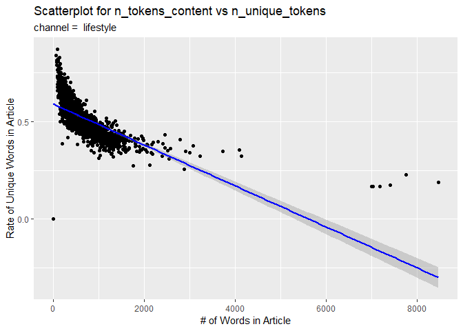
The second visual is a scatterplot with a trend line. The number of words in the content is on the x-axis and the rate of unique words on the y-axis. If the data points and trend line show an upward trend, then articles with more words tend to have a larger rate of unique ones. If there is a downward trend, then articles with more words tend to have a smaller rate of unique ones.
p <- ggplot(news.tbl, aes(x = n_tokens_content, y = n_unique_tokens))

p + geom_point() +
  geom_smooth(method = glm, col = "Blue") +
  labs(title = "Scatterplot for n_tokens_content vs n_unique_tokens",
       subtitle = paste("channel = ", params$channel),
       x = "# of Words in Article",
       y = "Rate of Unique Words in Article")
## `geom_smooth()` using formula 'y ~ x'
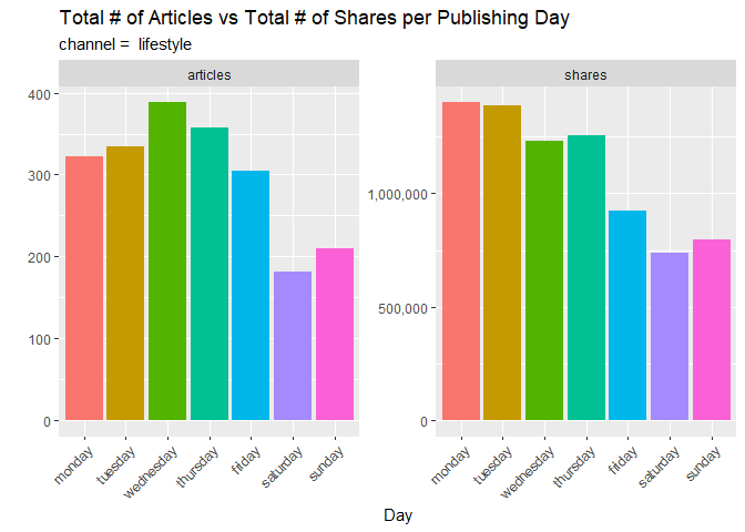
This subsequent bar plot shows a comparison between the total number of articles published on each day of the week and the total shares of those articles. Observe any interestingly sized columns that one might think would be higher or lower than others. Articles published on which day tend to get shared the most? Which one gets the least?
plt <- news.tbl %>% pivot_longer(cols = starts_with("weekday_is_"),
               names_to = "day",
               names_prefix = "weekday_is_",
               names_transform = as.factor,
               values_to = "count") %>%
  filter(count == 1) %>%
  select(-count, -starts_with("weekday_is_"))

#Reordering days
plt$day <- factor(plt$day,
    levels = c("monday", "tuesday", "wednesday", "thursday",
               "friday", "saturday", "sunday"))


plt <- plt %>%
  select(day, shares) %>%
  group_by(day) %>%
  summarise(articles = n(), shares = sum(shares))

plt <- reshape2::melt(plt, id.vars = c("day"))

p <- ggplot(plt, aes(x = day, y = value, fill = day))

p + geom_col() +
  facet_wrap(vars(variable), scales = "free") +
  scale_y_continuous(labels = scales::comma) +
  guides(x = guide_axis(angle = 45), fill = "none") +
  labs(title = "Total # of Articles vs Total # of Shares per Publishing Day",
       subtitle = paste("channel = ", params$channel),
       x = "Day",
       y = '')
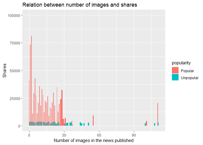
The code chunk below, tells us about the number of shares of a particular published news with number of images in the published news. It also tells us about the popularity of the news published with images.
ggplot(news.tbl, aes(fill= popularity, y=shares, x=num_imgs)) +
  geom_bar(position='dodge', stat='identity',  width = 0.98) +
  ggtitle('Relation between number of images and shares') +
  xlab('Number of images in the news published') +
  ylab('Shares') +
  ylim(0, 100000)
## Warning: Removed 3 rows containing missing values (geom_bar).
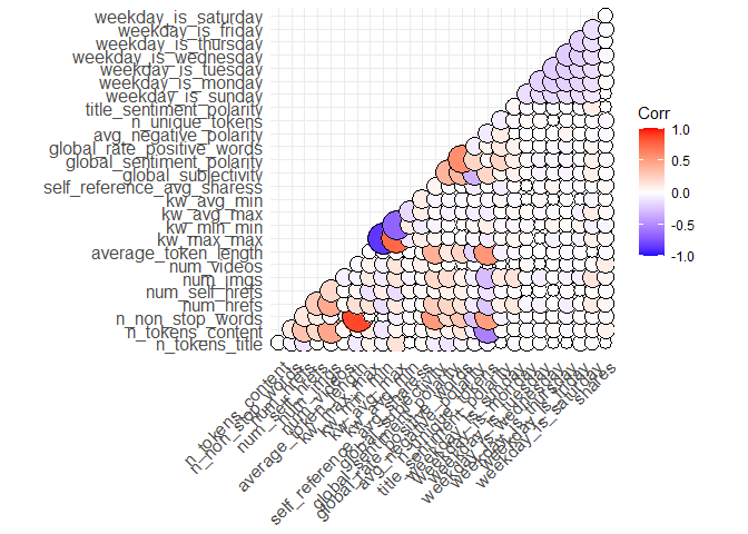
Correlation plots are used to find out the correlation between two
variables in the given data set. In the code chunk below, we have used
ggcorrplt() to plot the correlation between all the variables in the
data set and identify the most correlated variables. A violet
color circle shows there is negative correlation between the two
respective variables and a dark orange color is positive
correlation between two variables.
corr <- cor(select_if(news.tbl, is.numeric))

ggcorrplot(corr,
           method = "circle",
           type = "lower",
           outline.color = "black",
           lab_size = 6)
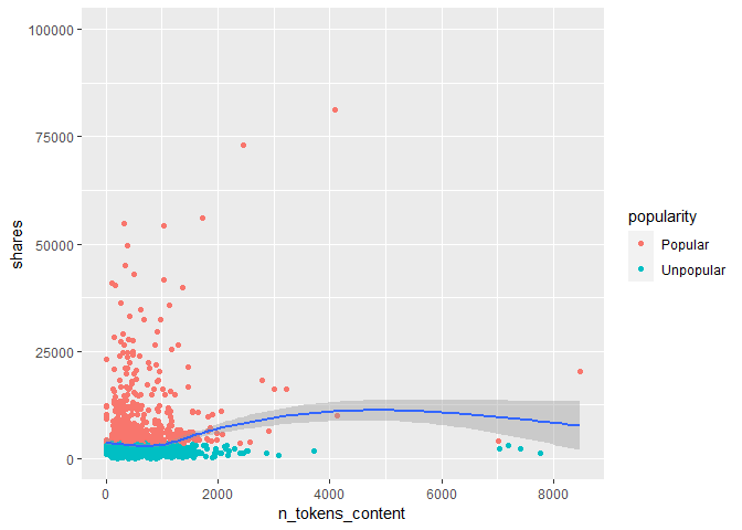
In the code chunk a scatter plot with a trend line. The number of words in the content is on the x-axis and the number of shares on the y-axis. If the data points and trend line show an upward trend, then articles with more words tend to have more number of shares. If there is a downward trend, then articles with more words tend to have a smaller number of shares.
ggplot(news.tbl, aes(y=shares, x=n_tokens_content)) +
    geom_point(aes(color=popularity)) +
    geom_smooth() +
    ylim(0, 100000)
## `geom_smooth()` using method = 'gam' and formula 'y ~ s(x, bs = "cs")'

## Warning: Removed 3 rows containing non-finite values (stat_smooth).

## Warning: Removed 3 rows containing missing values (geom_point).
Modeling
The goal now is to create models for predicting the number of shares
using linear regression and ensemble trees. Before that, the data is
split into a training (70%) and test (30%) set.
i <- createDataPartition(news.tbl[[1]], p = 0.7, list = FALSE)

train <- news.tbl[i,]
test <- news.tbl[-i,]
Linear Regression
Linear regression is a statistical technique that aims to demonstrate a relationship between variables. A dependent variable’s nature and degree of connection with a group of independent variables are assessed using linear regression. Symbolically: \(Y_i = \beta_0 + \beta_1 x_i + \epsilon_i\) where $Y_i$ is the dependent variable/response value, $\beta_0$ is the intercept, and $\beta_1$ is the slope coefficient for observation value $x_i$
We can make predictions of shares using linear regression models.
Model 1
The linear regression model is fit using variables chosen from forward
stepwise selection. The leaps library’s regsubsets() function performs
best subset selection by identifying the best model with a given number
of predictors, where best is quantified using $RSS$. The syntax is
identical to that of lm(). The summary() command returns the best set
of variables for each model size. In the code chunk below, we find the
best predictors subset, then $R^2$ value is used to determine the number
of predictors that can give best model results. Then we create a formula
that can be used to train the model by using as.formula() and
paste0().
fwdVars <- regsubsets(shares ~ ., train, method = "forward")
## Warning in leaps.setup(x, y, wt = wt, nbest = nbest, nvmax = nvmax, force.in = force.in, : 2 linear
## dependencies found

## Reordering variables and trying again:
fwdSumm <- summary(fwdVars)

adjRNum <- which.max(fwdSumm$adjr2)

bestModels <- fwdSumm$which[adjRNum,-1]

varNames <- names(which(bestModels == TRUE))

predictorFormulaPt2 <- paste(varNames, collapse = "+")

modelFormula <- as.formula(paste0("shares", "~", predictorFormulaPt2))

modelFormula
## shares ~ n_tokens_content + n_non_stop_words + num_hrefs + num_imgs +
##     self_reference_avg_sharess + global_subjectivity + n_unique_tokens +
##     title_sentiment_polarity + popularityUnpopular
## <environment: 0x00000204adee0e80>
In the code chunk below, firstly we have converted categorical variables
into numerical variables using dummyVars(). gsub() is used to rename
the column names in order to match with the column names generated by
regsubsets() in the function above. The caret package was used to
train a linear regression model by using the best predictors obtained
from regsubsets(). We have standardized the model using
center and scale. Cross validation is used to avoid over fitting and
add generalization in our model.
# convert categorical variables into numeric variables i.e one hot encoding
dummies <- dummyVars(shares ~ is_weekend+popularity, data = train)

trainDF <- as_tibble(predict(dummies, newdata = train)) %>%
    bind_cols(select(train,-is_weekend,-popularity))

# Replace . with spaces in column names to match the output names from regsubsets
names(trainDF) <- gsub(x = names(trainDF), pattern = "\\.", replacement = "")

forwardFit <- train(modelFormula,
                    data = trainDF,
                    method = "lm",
                    metric = "Rsquared",
                    preProcess = c("center","scale"),
                    trControl = trainControl(method = "cv", number = 10))

summary(forwardFit)
##
## Call:
## lm(formula = .outcome ~ ., data = dat)
##
## Residuals:
##    Min     1Q Median     3Q    Max
## -11522  -1081   -209    626 128999
##
## Coefficients:
##                            Estimate Std. Error t value Pr(>|t|)
## (Intercept)                  3461.0      143.5  24.124  < 2e-16 ***
## n_tokens_content             1030.9      225.7   4.568 5.34e-06 ***
## n_non_stop_words             -689.8      225.4  -3.060  0.00225 **
## num_hrefs                     259.0      169.4   1.529  0.12648
## num_imgs                     -513.6      183.7  -2.795  0.00525 **
## self_reference_avg_sharess    289.8      144.6   2.004  0.04522 *
## global_subjectivity           409.7      176.3   2.324  0.02028 *
## n_unique_tokens               644.5      240.1   2.684  0.00736 **
## title_sentiment_polarity      182.0      146.3   1.244  0.21362
## popularityUnpopular         -3482.4      145.7 -23.903  < 2e-16 ***
## ---
## Signif. codes:  0 '***' 0.001 '**' 0.01 '*' 0.05 '.' 0.1 ' ' 1
##
## Residual standard error: 5502 on 1461 degrees of freedom
## Multiple R-squared:  0.3025, Adjusted R-squared:  0.2982
## F-statistic:  70.4 on 9 and 1461 DF,  p-value: < 2.2e-16
Now we use the model to make predictions:
# convert categorical variables into numeric variables i.e one hot encoding
dummies <- dummyVars(shares ~ is_weekend+popularity, data = test)

testDF <- as_tibble(predict(dummies, newdata = test)) %>%
    bind_cols(select(test,-is_weekend,-popularity))

  predLR <- predict(forwardFit,newdata = testDF)

  predResultsFwd <- postResample(predLR,obs = testDF$shares)

  predResultsFwd
##         RMSE     Rsquared          MAE
## 1.181960e+04 1.592496e-01 2.665575e+03
Model 2
This second linear regression model is fit using variables chosen from backwards stepwise selection.
The regsubsets function is called, and the summary is returned to grab
the models of $n$ terms that have the optimal values for $R^2$, Mallows’
Cp, and BIC. As performance will vary, the mode value between the three
is chosen as the ‘best’.
backVars <- regsubsets(shares ~ ., train, method = "backward")
## Warning in leaps.setup(x, y, wt = wt, nbest = nbest, nvmax = nvmax, force.in = force.in, : 2 linear
## dependencies found

## Reordering variables and trying again:
backSumm <- summary(backVars, all.best = FALSE)

met <- c(R2 = which.max(backSumm$rsq),
     Cp = which.min(backSumm$cp),
     BIC = which.min(backSumm$bic)
)

M <- which.max(tabulate(met))
The most frequent number is 2. The variables present in this size model are:
terms <- coef(backVars, M)
terms
##         (Intercept)    n_tokens_content weekday_is_saturday
##         2612.919448            1.226932          935.405737
Now, the model can be trained. The coefficient names are grabbed from the backwards selection, and input as a subset of the training data. The variables are standardized to account for the vastly different magnitudes between them, and to prevent any extreme coefficient values because of this.
prd <- names(terms)

#Assuming these terms appear in the model, but just a warning otherwise
prd <- replace(prd, prd %in% c('(Intercept)', 'is_weekend1'), c('shares', 'is_weekend'))
## Warning in x[list] <- values: number of items to replace is not a multiple of replacement length
BackwardFit <- train(shares ~ .,
                    data = train[,prd],
                    method = "lm",
                    metric = "Rsquared",
                    preProcess = c("scale", "center"),
                    trControl = trainControl(method = "cv", number = 10))

summary(BackwardFit)
##
## Call:
## lm(formula = .outcome ~ ., data = dat)
##
## Residuals:
##    Min     1Q Median     3Q    Max
## -10839  -2297  -1623    -59 135953
##
## Coefficients:
##                     Estimate Std. Error t value Pr(>|t|)
## (Intercept)           3461.0      170.2  20.340  < 2e-16 ***
## n_tokens_content       732.5      170.2   4.303 1.79e-05 ***
## weekday_is_saturday    259.0      170.2   1.522    0.128
## ---
## Signif. codes:  0 '***' 0.001 '**' 0.01 '*' 0.05 '.' 0.1 ' ' 1
##
## Residual standard error: 6526 on 1468 degrees of freedom
## Multiple R-squared:  0.01409,    Adjusted R-squared:  0.01274
## F-statistic: 10.49 on 2 and 1468 DF,  p-value: 3.001e-05
The model is then tested against the testing data:
predLRBck <- predict(BackwardFit, newdata = test)

predResultsBck <- postResample(predLRBck, obs = test$shares)
predResultsBck
##         RMSE     Rsquared          MAE
## 1.276719e+04 5.124393e-04 3.806488e+03
Random Forest
Random forest uses the same idea as bagging tree models. It is a bootstrap aggregation method, but the difference is that random forests randomly select a subset of predictors instead of using all the predictors. This is because if a really strong predictor exists, every bootstrap tree will probably use it for the first split. This will result in making bagged trees predictions more correlated, and variance will be large in aggregation. Hence, in random forest we avoid this limitation by using a random subset of predictors for each bootstrap sample/tree fit.
In the code chunk below, caret package was used to train the rf forest
model and the evaluation metric used for the fit is Rsquared. We have
tuned the model by using tuning parameter mtry ad used 5 folds cross
validation for finding best fit.
#5 folds cross validation
control <- trainControl(method='cv',
                        number=5)

tunegrid <- data.frame(mtry = 1:9)
rfFit <- train(modelFormula,
                      data=trainDF,
                      method='rf',
                      metric='Rsquared',
                      tuneGrid=tunegrid,
                      trControl=control)

rfFit$bestTune
##   mtry
## 1    1
varImp(rfFit$finalModel) %>% arrange(desc(Overall))
##                                Overall
## popularityUnpopular        11419515376
## n_tokens_content            5305051740
## n_non_stop_words            5292824672
## n_unique_tokens             5098958477
## global_subjectivity         4214475229
## self_reference_avg_sharess  3980129969
## num_hrefs                   3622387761
## title_sentiment_polarity    2295335742
## num_imgs                    2285355548
# convert categorical variables into numeric variables i.e one hot encoding
dummies <- dummyVars(shares ~ is_weekend+popularity, data = test)

testDF <- as_tibble(predict(dummies, newdata = test)) %>%
    bind_cols(select(test,-is_weekend,-popularity))

predRF <- predict(rfFit,newdata = testDF)

predResultsRF <- postResample(predRF,obs = testDF$shares)
predResultsRF
##         RMSE     Rsquared          MAE
## 12012.047387     0.159827  2688.797658
Boosted Tree Model
Boosting centers around the idea of sequential learning–taking information from preceding iterations as a basis for calculating the current iteration. Boosted trees are ensemble tree models consisting of a group of trees that are built in sequence, including errors from previous trees for predictions.
Boosted trees also have a unique characteristic of slow training. This
is controlled by $\lambda$, a shrinkage parameter. The two other notable
parameters for training a boosted tree are $B$ (the number of times the
algorithm performs its procedure; n.trees in R) and $d$ (the number of
splits; interaction.depth in R), both of which can be selected with
cross-validation.
For regression, the boosting algorithm proceeds as follows:
- The predictions are initialized to 0–$\hat{y}(x)=0$
- The residuals between observed and predicted values are calculated
- A tree with $d$ splits and $d+1$ terminal nodes is fit using the residuals as the response–denoted by $\hat{y}^b(x)$
- The overall prediction is updated by recursively adding these pseudo-responses–$\hat{y}(x) +=\lambda\hat{y}^b(x)$
- Residuals for new predictions are updated
- Repeat $B$ times
This model is fit using cv = 10, and the train function will
determine the optimal values of the parameters for us.
#Output for this chunk is hidden as it is rather long and does not provide information needed for reporting
boostFit <- train(shares ~ .,
              method = "gbm",
              data = train,
              trControl = trainControl(method = "cv", number = 10))
During training, the optimal values for the tuning parameters were found to be:
boostFit$bestTune
##   n.trees interaction.depth shrinkage n.minobsinnode
## 1      50                 1       0.1             10
Since coefficients aren’t interpretable for boosted trees, the calculation of variable importance for the final model is shown instead, in descending order:
varImp(boostFit$finalModel) %>% arrange(desc(Overall))
##                                Overall
## popularityUnpopular        51169008680
## n_non_stop_words            5569097821
## self_reference_avg_sharess  4125956531
## num_hrefs                   1045059242
## n_tokens_content             734582191
## global_subjectivity          346058329
## kw_avg_min                   275110211
## n_unique_tokens              233513738
## global_rate_positive_words   233369062
## kw_avg_max                   155221150
## num_imgs                      98932398
## n_tokens_title                       0
## num_self_hrefs                       0
## num_videos                           0
## average_token_length                 0
## kw_max_max                           0
## kw_min_min                           0
## is_weekend1                          0
## global_sentiment_polarity            0
## avg_negative_polarity                0
## title_sentiment_polarity             0
## weekday_is_sunday                    0
## weekday_is_monday                    0
## weekday_is_tuesday                   0
## weekday_is_wednesday                 0
## weekday_is_thursday                  0
## weekday_is_friday                    0
## weekday_is_saturday                  0
Now, the results of applying the boosted tree to the test data:
predBoost <- predict(boostFit,newdata = test)

predResultsBoost <- postResample(predBoost,obs = test$shares)
predResultsBoost
##         RMSE     Rsquared          MAE
## 1.189679e+04 1.554667e-01 2.564866e+03
Model Comparison
The metric results of each model are returned in the table below. The metric that they are “judged” against is RMSE, and the model with the minimum value is the “winner”.
rmseModels <- c(predResultsFwd[[1]],predResultsBck[[1]],
                predResultsRF[[1]],predResultsBoost[[1]])

modelName <- c("Linear Regression (Forward Var. Selection)", "Linear Regression (Backward Var. Selection)",
               "Random foresF", "Boosted Tree")

resultsDF <- tibble(modelName, rmseModels)
resultsDF
## # A tibble: 4 × 2
##   modelName                                   rmseModels
##   <chr>                                            <dbl>
## 1 Linear Regression (Forward Var. Selection)      11820.
## 2 Linear Regression (Backward Var. Selection)     12767.
## 3 Random foresF                                   12012.
## 4 Boosted Tree                                    11897.
bestModelName <- filter(resultsDF,rmseModels == min(rmseModels))[[1]]

paste0("The best model for the ", params$channel, " channel is: ", bestModelName)
## [1] "The best model for the lifestyle channel is: Linear Regression (Forward Var. Selection)"